.

In this tutorial, I’ll guide you through the process of extracting polygons from a raster file using a specific land class defined by its RGB values. We will also generate random points within those polygons. This guide is perfect for those working with land cover classifications and interested in visualizing specific land use categories—like the Single Crop class—on a map.

What We’ll Cover:

• Extracting polygons from raster data based on specific RGB values.
• Generating random points within the extracted polygons.
• Visualizing the shapefiles and creating a feature image for your project.

Tools and Libraries:

We will use several Python libraries for this task:

• rasterio: To read and process the raster file.
• shapely: To handle the geometrical aspects of the shapes.
• fiona: To write shapefiles.
• geopandas: To work with geospatial data and generate random points.
• matplotlib: For visualization of the shapefiles.

Let's jump right in!

1. Understanding the Data

Land cover classification maps usually encode different land types using specific RGB values. In our example, the Single Crop land cover class is represented by the RGB value (254, 239, 187).

We will use this RGB value to extract the Single Crop polygons from the raster file and then generate random points inside the polygons.

2. Setting Up the Environment

Before we start coding, install the required libraries. You can install them using pip:

pip install rasterio shapely geopandas fiona matplotlib

Once installed, you’re ready to start working with the code.

3. Extracting Polygons from the Raster File

Step 1: Loading the Raster File

The first step is to load your raster file (.tif) and locate areas matching the RGB value for Single Crop.

import numpy as np
import rasterio
from rasterio.features import shapes
from shapely.geometry import shape, mapping
import fiona
from fiona.crs import from_epsg
import os

class SingleCropShapefileGenerator:
    def __init__(self, file_path, target_rgb=(254, 239, 187)):
        self.file_path = file_path
        self.target_rgb = target_rgb

    def classify(self):
        # Open the TIFF file
        with rasterio.open(self.file_path) as src:
            # Read the bands as arrays (assuming it's RGB)
            r = src.read(1)  # Red band
            g = src.read(2)  # Green band
            b = src.read(3)  # Blue band
            
            # Stack the bands to form an RGB array
            rgb = np.stack([r, g, b], axis=-1)
            
            # Create a boolean mask where the RGB values match the target
            mask = np.all(rgb == self.target_rgb, axis=-1)
            
            return mask, src.transform, src.crs

    def generate_shapefile(self, output_shp):
        mask, transform, crs = self.classify()
        
        # Convert the mask into shapes (polygons)
        shapes_gen = shapes(mask.astype(np.uint8), transform=transform)

        # Define schema for shapefile (geometry type: Polygon)
        schema = {
            'geometry': 'Polygon',
            'properties': {'category': 'str'}
        }
        
        # Write the shapes (polygons) to a shapefile
        with fiona.open(output_shp, 'w', driver='ESRI Shapefile', crs=crs.to_dict(), schema=schema) as shp:
            for geom, value in shapes_gen:
                if value:  # Only take shapes where the mask is True
                    shp.write({
                        'geometry': mapping(shape(geom)),
                        'properties': {'category': 'Single Crop'}
                    })

# Usage
file_path = '/path/to/your/raster/BDLC2015.tif'  # Path to your TIFF file
output_shp = '/path/to/save/single_crop.shp'  # Path to save the shapefile
output_dir = '/path/to/save/directory/'
if not os.path.exists(output_dir):
    os.makedirs(output_dir)

output_shp = os.path.join(output_dir, 'single_crop.shp')
single_crop_generator = SingleCropShapefileGenerator(file_path)
single_crop_generator.generate_shapefile(output_shp)

4. Generating Random Points within the Extracted Polygons

Now that we have the Single Crop polygons, let's generate random points inside these polygons.

Step 2: Generate Random Points

import geopandas as gpd
from shapely.geometry import Point
import random

def generate_random_points(shapefile_path, num_points=10, output_csv=None):
    # Load the shapefile
    gdf = gpd.read_file(shapefile_path)
    
    # Create an empty list to hold random points
    points = []
    
    # Generate random points inside the polygons
    for _ in range(num_points):
        while True:
            # Choose a random polygon from the GeoDataFrame
            polygon = gdf.sample(1).geometry.values[0]
            
            # Generate a random point inside the bounding box of the polygon
            minx, miny, maxx, maxy = polygon.bounds
            point = Point(random.uniform(minx, maxx), random.uniform(miny, maxy))
            
            # Check if the point is within the polygon
            if polygon.contains(point):
                points.append((point.x, point.y))
                break
    
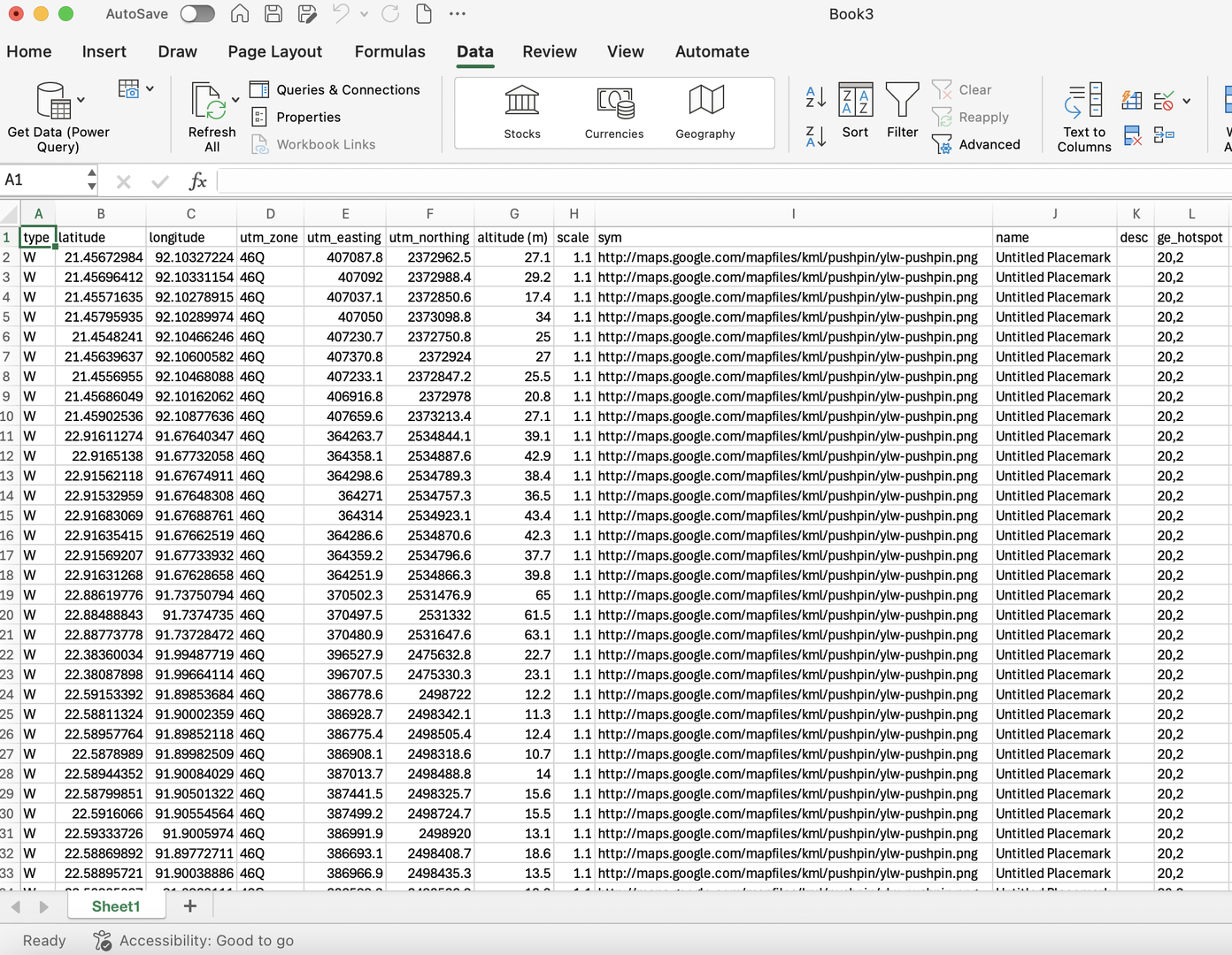
    # Save the points to a CSV file
    if output_csv:
        np.savetxt(output_csv, points, delimiter=',', header="Longitude,Latitude", comments='')
        print(f"Random points saved to {output_csv}")
    
    return points

# Usage
shapefile_path = '/path/to/save/single_crop.shp'
output_csv = '/path/to/save/single_crop_random_points.csv'
generate_random_points(shapefile_path, num_points=20, output_csv=output_csv)

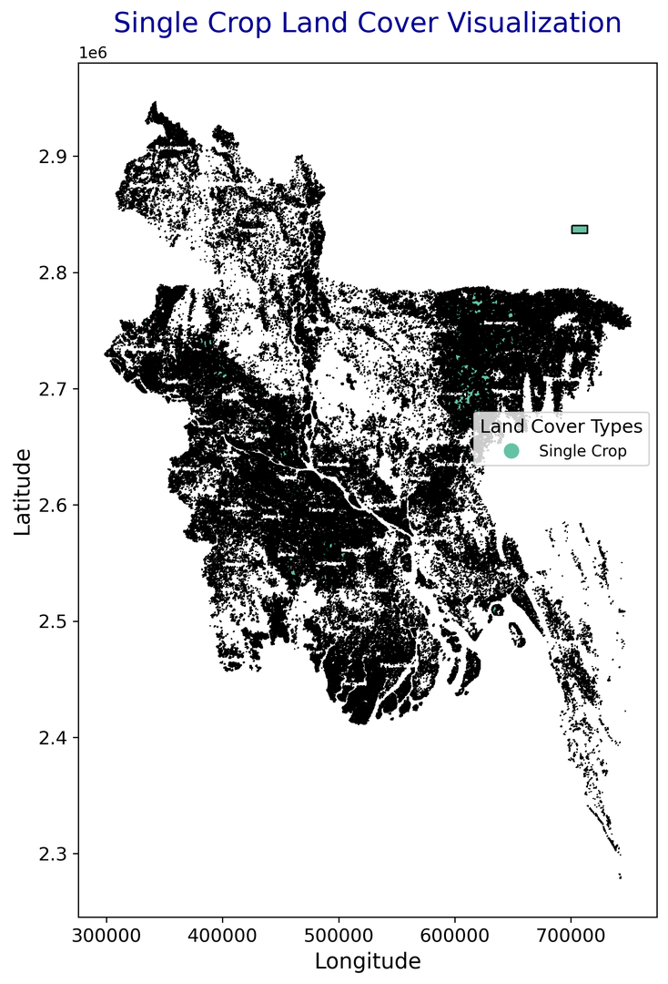
5. Visualizing the Shapefile

To create a feature image for your blog post, we’ll plot the shapefile in Python using GeoPandas and Matplotlib.

import geopandas as gpd
import matplotlib.pyplot as plt
from mpl_toolkits.axes_grid1 import make_axes_locatable

def plot_shapefile_enhanced(shapefile_path, title="Single Crop Land Cover", output_image_path=None):
    # Load the shapefile into a GeoDataFrame
    gdf = gpd.read_file(shapefile_path)

    # Create the figure and axis
    fig, ax = plt.subplots(1, 1, figsize=(12, 10))

    # Choose a colorful colormap
    cmap = 'Set2'
    
    # Plot the shapefile with polygons filled with vibrant colors
    gdf.boundary.plot(ax=ax, linewidth=1, color='black')
    gdf.plot(ax=ax, column='category', cmap=cmap, legend=True, edgecolor='black')

    # Customize the legend
    leg = ax.get_legend()
    leg.set_bbox_to_anchor((1, 0.6))  # Position the legend outside the plot
    leg.set_title("Land Cover Types", prop={'size': 12})

    # Set the title and axis labels with more prominent fonts
    ax.set_title(title, fontsize=18, pad=20, color='darkblue')
    ax.set_xlabel("Longitude", fontsize=14)
    ax.set_ylabel("Latitude", fontsize=14)

    # Save or display the image
    if output_image_path:
        plt.savefig(output_image_path, dpi=300, bbox_inches='tight', transparent=True)
        print(f"Image saved to {output_image_path}")
    else:
        plt.show()

# Usage
shapefile_path = '/path/to/save/single_crop.shp'
output_image_path = '/path/to/save/single_crop_visualization_enhanced.png'
plot_shapefile_enhanced(shapefile_path, title="Single Crop Land Cover Visualization", output_image_path=output_image_path)

Conclusion

By following these steps, you can easily extract specific land cover classes from a raster file using RGB values and visualize them as polygons. Additionally, you can generate random points inside those polygons, which can be useful for sampling and analysis tasks.

Feel free to experiment with other land cover categories by adjusting the RGB values. If you have any questions or suggestions, leave a comment below!