.

Geospatial data often comes with various Coordinate Reference Systems (CRS), which define how coordinates are mapped to locations on Earth's surface. Changing the CRS of a shapefile is crucial for ensuring accurate spatial analysis and visualization. In this tutorial, we'll explore how to manage CRS transformations using Python and Jupyter Notebook, focusing on converting a shapefile to a different projection system.

Step 1: Importing Libraries, Read Shapefile and checking Original CRS

import geopandas as gpd
from pyproj import CRS
import matplotlib.pyplot as plt

# Read the shapefile (set CRS explicitly if needed)
gdf = gpd.read_file('/home/manik/Documents/pygis/district/district.shp')

# Check the original CRS
print("Original CRS:", gdf.crs)

Step 2: Setting CRS Explicitly (if needed)

# Set CRS explicitly to WGS84 (EPSG:4326) if it's None
if gdf.crs is None:
    gdf.crs = CRS.from_epsg(4326)
    print("Updated CRS to WGS84:", gdf.crs)
else:
    print("Original CRS:", gdf.crs)

Step 3: Converting to a New CRS and Saving the Converted Shapefile

import os

# Convert to UTM Zone 45N (EPSG:32645)
gdf_utm = gdf.to_crs(epsg=32645)

# Check the new CRS
print("Converted CRS to UTM Zone 45N:", gdf_utm.crs)

# Specify the output folder path
output_folder = '/home/manik/Documents/pygis/proj_utm_45N/'

# Create the folder if it doesn't exist
os.makedirs(output_folder, exist_ok=True)

# Save the converted GeoDataFrame to a new shapefile in the specified folder
gdf_utm.to_file(output_folder + 'converted_shapefile_utm.shp')

# Save as GeoJSON or other formats supported by GeoPandas
gdf_utm.to_file(output_folder + 'converted_shapefile_utm.geojson', driver='GeoJSON')

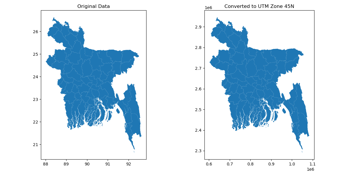
Step 4: Visualization (Optional)

# Plot to visualize the data
import matplotlib.pyplot as plt

fig, (ax1, ax2) = plt.subplots(1, 2, figsize=(12, 6))

# Plot original data
ax1.set_title('Original Data')
gdf.plot(ax=ax1)

# Plot converted data
ax2.set_title('Converted to UTM Zone 45N')
gdf_utm.plot(ax=ax2)

plt.tight_layout()
plt.show()

Step 5: Save Visualized image 

# Create a figure and subplots
fig, (ax1, ax2) = plt.subplots(1, 2, figsize=(12, 6))

# Plot original data
ax1.set_title('Original Data')
gdf.plot(ax=ax1)

# Plot converted data
ax2.set_title('Converted to UTM Zone 45N')
gdf_utm.plot(ax=ax2)

# Adjust layout for better visualization
plt.tight_layout()

# Save the plot as an image file (PNG format in this example)
plt.savefig(output_folder + 'visualization.png')

# Show the plot (optional)
plt.show()