Elevation Mapping in Southern Bangladesh: A Step-by-Step Guide

In this blog post, we will walk through the entire process of cropping a shapefile based on a specified area and visualizing the elevation data of Southern Bangladesh. We will use Python's GeoPandas and Matplotlib libraries to achieve this.

Step 1: Setting Up Your Environment

Before we start, make sure you have the following libraries installed:

pip install geopandas matplotlib

You will also need shapefiles for the area of interest and the elevation data. For this guide, we'll be using:

Crop Area Shapefile: southbd.shp
Elevation Shapefile: bgd_elev.shp

These files should be stored in accessible directories.

Step 2: Loading the Shapefiles

We begin by loading the necessary shapefiles using GeoPandas.

import geopandas as gpd

# Load the shapefiles
crop_area = gpd.read_file(r'C:\Users\SARKER\Downloads\southernpart\southbd.shp')
shapefile_to_crop = gpd.read_file(r'C:\Users\SARKER\Downloads\bgd_elevation\bgd_elev.shp')

Step 3: Aligning Coordinate Reference Systems (CRS)

It’s essential that both shapefiles use the same CRS. We can check and align them as follows:

# Check and align CRS if necessary
if crop_area.crs != shapefile_to_crop.crs:
    shapefile_to_crop = shapefile_to_crop.to_crs(crop_area.crs)

Step 4: Cropping the Shapefile

Next, we crop the elevation shapefile to the specified area defined by the crop shapefile using the overlay function:

# Crop the shapefile
cropped_shapefile = gpd.overlay(shapefile_to_crop, crop_area, how='intersection')

Step 5: Saving the Cropped Shapefile

To keep our workspace organized, we save the cropped shapefile:

output_directory = r'C:\Users\SARKER\Downloads\cropped_shapefile'
os.makedirs(output_directory, exist_ok=True)

if not cropped_shapefile.empty:
    output_path = os.path.join(output_directory, 'cropped_shapefile.shp')
    cropped_shapefile.to_file(output_path)

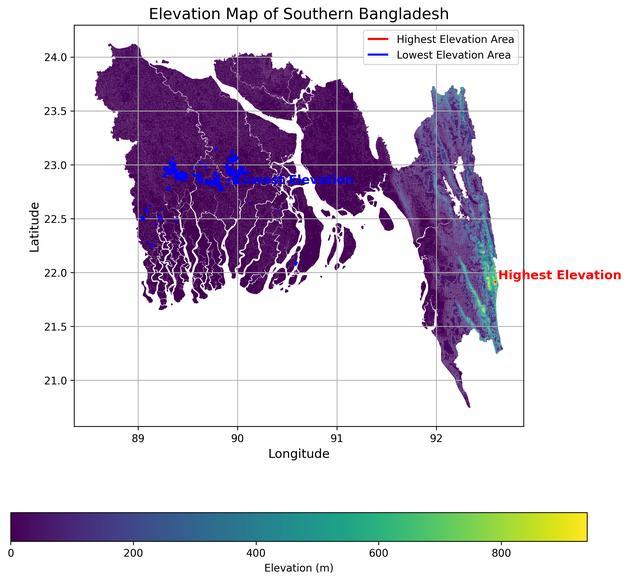
Step 6: Visualizing Elevation Data

Now that we have our cropped shapefile, we can visualize the elevation data. We will create a plot that displays the elevation values clearly, marking the highest and lowest elevation areas.

import matplotlib.pyplot as plt

# Load the cropped shapefile
cropped_shapefile = gpd.read_file(output_path)

# Find the highest and lowest elevation
highest_elevation = cropped_shapefile['elev_m'].max()
lowest_elevation = cropped_shapefile['elev_m'].min()

highest_geom = cropped_shapefile[cropped_shapefile['elev_m'] == highest_elevation].geometry
lowest_geom = cropped_shapefile[cropped_shapefile['elev_m'] == lowest_elevation].geometry

# Plot the cropped shapefile with elevation
fig, ax = plt.subplots(1, 1, figsize=(10, 10))
cropped_shapefile.plot(column='elev_m', cmap='viridis', legend=True, ax=ax)

# Mark the highest and lowest elevation areas
if not highest_geom.empty:
    highest_geom.boundary.plot(ax=ax, color='red', linewidth=2)
    ax.annotate('Highest Elevation', xy=highest_geom.centroid.iloc[0].coords[0],
                xytext=(3, 3), textcoords="offset points", color='red', fontsize=12)

if not lowest_geom.empty:
    lowest_geom.boundary.plot(ax=ax, color='blue', linewidth=2)
    ax.annotate('Lowest Elevation', xy=lowest_geom.centroid.iloc[0].coords[0],
                xytext=(-10, -10), textcoords="offset points", color='blue', fontsize=12)

# Customize the plot
plt.title('Elevation Map of Southern Bangladesh', fontsize=15)
plt.xlabel('Longitude', fontsize=12)
plt.ylabel('Latitude', fontsize=12)
plt.grid(True)

# Save the plot as an image
output_image_path = r'C:\Users\SARKER\Downloads\elevation_map_southern_bangladesh.png'
plt.savefig(output_image_path, bbox_inches='tight', dpi=300)
plt.show()

Here's the complete code consolidated into one file. This script will load the shapefiles, crop the elevation data, and visualize the elevation map while saving the final image.

import geopandas as gpd
import os
import matplotlib.pyplot as plt

# Load the shapefiles
crop_area_path = r'C:\Users\SARKER\Downloads\southernpart\southbd.shp'
shapefile_to_crop_path = r'C:\Users\SARKER\Downloads\bgd_elevation\bgd_elev.shp'

crop_area = gpd.read_file(crop_area_path)
shapefile_to_crop = gpd.read_file(shapefile_to_crop_path)

# Check and align CRS if necessary
if crop_area.crs != shapefile_to_crop.crs:
    shapefile_to_crop = shapefile_to_crop.to_crs(crop_area.crs)

# Crop the shapefile
cropped_shapefile = gpd.overlay(shapefile_to_crop, crop_area, how='intersection')

# Define the output directory for cropped shapefile
output_directory = r'C:\Users\SARKER\Downloads\cropped_shapefile'
os.makedirs(output_directory, exist_ok=True)

# Save the cropped shapefile if it's not empty
if not cropped_shapefile.empty:
    output_path = os.path.join(output_directory, 'cropped_shapefile.shp')
    cropped_shapefile.to_file(output_path)
else:
    print("The cropped shapefile is empty. No file saved.")

# Load the cropped shapefile for visualization
cropped_shapefile = gpd.read_file(output_path)

# Find the highest and lowest elevation
if 'elev_m' in cropped_shapefile.columns:
    highest_elevation = cropped_shapefile['elev_m'].max()
    lowest_elevation = cropped_shapefile['elev_m'].min()
    
    # Get geometries for highest and lowest elevations
    highest_geom = cropped_shapefile[cropped_shapefile['elev_m'] == highest_elevation].geometry
    lowest_geom = cropped_shapefile[cropped_shapefile['elev_m'] == lowest_elevation].geometry

    print(f"Highest Elevation: {highest_elevation} m")
    print(f"Lowest Elevation: {lowest_elevation} m")
else:
    print("The 'elev_m' column is not found in the attribute table.")

# Plot the cropped shapefile with elevation
fig, ax = plt.subplots(1, 1, figsize=(10, 10))
cropped_shapefile.plot(column='elev_m', cmap='viridis', legend=True,
                       legend_kwds={'label': "Elevation (m)",
                                    'orientation': "horizontal"},
                       ax=ax)

# Mark the highest and lowest elevation areas
if not highest_geom.empty:
    highest_geom.boundary.plot(ax=ax, color='red', linewidth=2, label='Highest Elevation Area')
    ax.annotate('Highest Elevation', xy=highest_geom.centroid.iloc[0].coords[0],
                xytext=(3, 3), textcoords="offset points", color='red',
                fontsize=12, fontweight='bold')

if not lowest_geom.empty:
    lowest_geom.boundary.plot(ax=ax, color='blue', linewidth=2, label='Lowest Elevation Area')
    ax.annotate('Lowest Elevation', xy=lowest_geom.centroid.iloc[0].coords[0],
                xytext=(-10, -10), textcoords="offset points", color='blue',
                fontsize=12, fontweight='bold')

# Customize the plot
plt.title('Elevation Map of Southern Bangladesh', fontsize=15)
plt.xlabel('Longitude', fontsize=12)
plt.ylabel('Latitude', fontsize=12)
plt.grid(True)
plt.legend()

# Save the plot as an image
output_image_path = r'C:\Users\SARKER\Downloads\elevation_map_southern_bangladesh.png'
plt.savefig(output_image_path, bbox_inches='tight', dpi=300)  # Save image with high resolution
plt.show()

print(f"Elevation map saved successfully at: {output_image_path}")

Conclusion

In this guide, we have successfully cropped a shapefile based on a specified area and visualized the elevation data of Southern Bangladesh. The final image not only displays the elevation but also highlights the areas of highest and lowest elevation.

Feel free to customize the code further to meet your specific needs or to explore additional features in your data. Happy coding!

Gis & rs

.